Automated exploratory data analysis in R
You want to listen to what your data tells you. But that can be hard when you have a lot of things (variables) you’re keeping track of. If you measure 10 variables and are interested in what’s happening in your dataset, you need to produce at least 10 choose 2 = 45 plots. That’ll take some time. If there are 20 variables, creating 190 plots is in your future. But your outlook is improving with the code I’m sharing below.
The goal of the eda function is to allow you to quickly get a sense of potential patterns in your dataset that you can then follow up on with a more thorough analysis.
what it does
The eda function, the code for which you can find here, computes some statistic of interest between every pair of columns in your dataframe. The statistic it computes depends on the nature of the variables:
-
We calculate the correlation coefficient for two continuous variables. A correlation, or r, ranges from -1 to 1. Values near zero are rarely interesting.
-
Goodman and Kruskal’s tau is calculated if the two variables are both categorical. It can range from 0 (not interesting) to 1 (interesting).
Interestingly, tau is not symmetric: tau(x,y) is not necessarily the same as tau(y,x). Why? Think of the relationship between country and continent, two categorical variables. If I know the country, I know with 100% certainty what continent it belongs to. So tau(country, continent) is 1. But if I’m only given the continent and had to predict the country, I’d have a harder time (except for Australia or Antarctica). So tau(continent, country) < 1, for the ability for continent to predict country is less than perfect.
- Finally, for the relationship between a categorical and a continuous variable, we calculate the intraclass correlation coefficient, or ICC. It ranges from 0 (not interesting) to 1 (interesting).
The eda function figures out the appropriate test to use for each pair of variables.
the input
The input to the eda (which stands for ‘exploratory data analysis’, by the way) is a dataframe. The function assumes that each thing you care about, i.e., each variable, is in its own column. If not, you’ll need to gather or spread with tools from the tidyr package. It also assumes that categorical variables are coded as factors in R. You can check this with the is.factor function. Character vectors are simply ignored.
the output
The output is also a dataframe. The dataframe has six columns:
- var1: the first variable
- var2: the second variable
- statistic: what type of statistic was calculated (r, the ICC, or tau).
- value: the value of the statistic
- p_value: p-value for the relationship. Based on permutation tests with only 99 permutations for tau and ICC for speed reasons. Take with a grain of salt or a whole box of Morton’s. As explained elsewhere, the purpose of this function is to give you a sense of interesting or strong relationships in your data, not to give you a final result.
- n: the number of observations. This might vary due to missingness in some columns. By default, missing values are removed.
let’s try it out
We can source the function, or load it so that R recognizes it, from the web:
source("https://raw.githubusercontent.com/lukereding/random_scripts/master/eda.R")
If you try to use the function without installing the tidyverse, GoodmanKruskal, or ICC libraries, you will likely run into problems. If you don’t have one of these libraries, use install.packages like install.packages("ICC"). If you aren’t sure, you can see what library("ICC") returns or simply re-install the package.
Let’s see what this function returns on the fabled iris dataset:
library(tidyverse)

data(iris)

# make sure species is a factor
iris$Species <- factor(iris$Species)

eda(iris)
A tibble: 10 x 6
           var1         var2 statistic      value      p_value     n
          <chr>        <chr>     <chr>      <dbl>        <dbl> <int>
 1 Sepal.Length  Sepal.Width         r -0.1175698 1.518983e-01   150
 2 Sepal.Length Petal.Length         r  0.8717538 1.038667e-47   150
 3 Sepal.Length  Petal.Width         r  0.8179411 2.325498e-37   150
 4 Sepal.Length      Species       ICC  0.7028488 1.000000e-02   150
 5  Sepal.Width Petal.Length         r -0.4284401 4.513314e-08   150
 6  Sepal.Width  Petal.Width         r -0.3661259 4.073229e-06   150
 7  Sepal.Width      Species       ICC  0.4906278 1.000000e-02   150
 8 Petal.Length  Petal.Width         r  0.9628654 4.675004e-86   150
 9 Petal.Length      Species       ICC  0.9593219 1.000000e-02   150
10  Petal.Width      Species       ICC  0.9504463 1.000000e-02   150
As promised, a dataframe with six columns. From here, it might be nice to make a plot so that we can visually see the more interesting relationships.
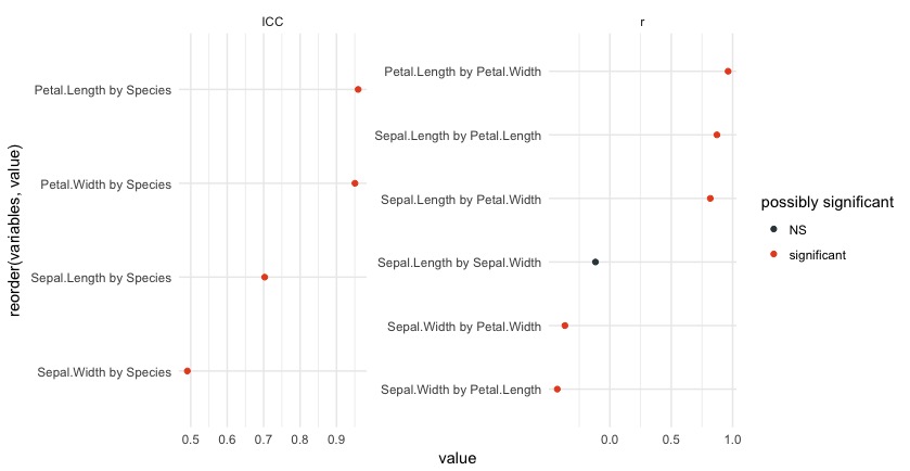
You can produce a plot quickly by setting plot = TRUE in eda:
eda(iris, plot = TRUE)
Or we can create it like this:
eda(iris) %>%
  unite(combo, var1, var2, sep = " by ") %>% # make a new column with the combination of both variables
  mutate(`possibly significant` = if_else(p_value < 0.05, "significant", "NS")) %>%
  ggplot(aes(x = reorder(combo, value), y = value, color = `possibly significant`)) +
  geom_point() +
  facet_wrap(~statistic, scales = "free") +
  coord_flip() +
  theme_minimal()
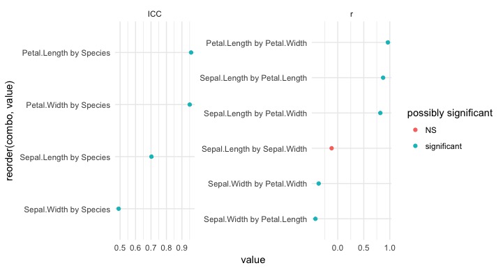
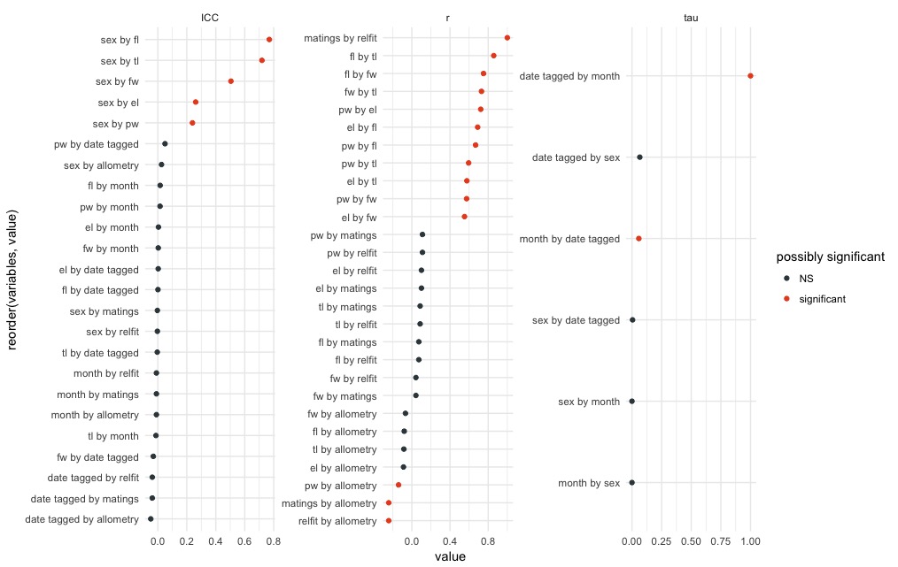
This plot is pretty informative. The ICC side of the plot contains relationships between categorcial and continuous variables, while the plot on the right contains relationships between continuous variables.
One thing we see is that Species and Petal.Length have a high ICC. We can plot this relationship to verify this:
iris %>%
  ggplot(aes(x = Species, y = Petal.Length)) +
  geom_jitter(width = 0.1) +
  theme_minimal()
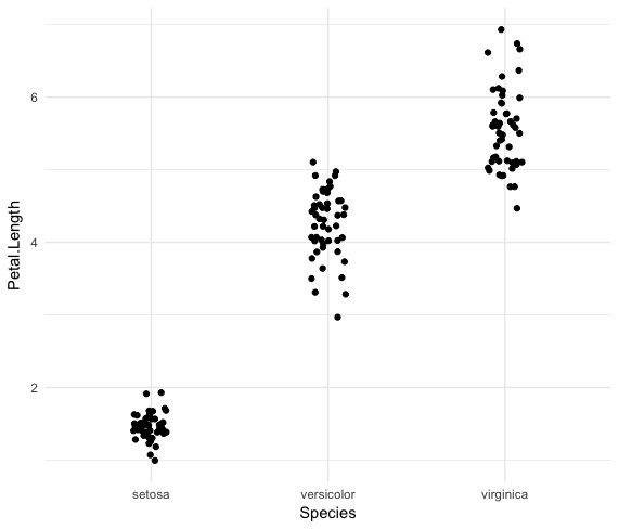
Petal length differs a lot between species and relatively little within a species, giving rise to the high ICC value.
The relationship between Sepal.Width and Species is less strong; it looks like this:
iris %>%
  ggplot(aes(x = Species, y = Sepal.Width)) +
  geom_jitter(width = 0.1) +
  theme_minimal()
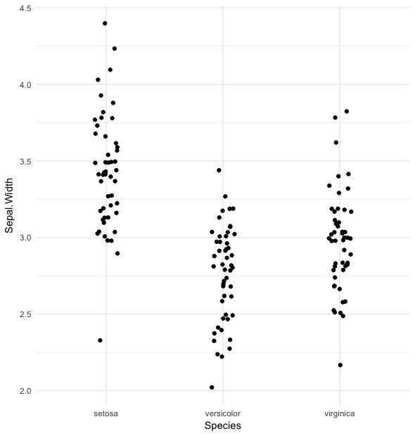
There’s still some separation here, but it’s clear it’s not as strong as the previous relationship.
one more time
Let’s try a different dataset:
x <- read_csv("http://datadryad.org/bitstream/handle/10255/dryad.154475/mating_success_allometry_2014.csv?sequence=1")

head(x)
A tibble: 6 x 12
  number   sex    pw    el    fl    fw    tl month `date tagged`
   <chr> <chr> <dbl> <dbl> <dbl> <dbl> <dbl> <int>         <int>
1     w1     m   4.0  12.4  10.2   3.4   8.3     7            21
2     w2     f   3.3  12.2   6.8   2.8   5.4     7            21
3     w3     m   4.1  14.8  10.8   3.7   9.3     7            21
4     w4     f   3.8  12.4   6.5   2.8   5.2     7            21
5     w5     m   4.0  13.3  10.2   3.5   8.1     7            21
6     w6     f   3.4  11.2   5.8   2.6   5.4     7            21
	# ... with 3 more variables: matings <int>, relfit <dbl>,
	#   allometry <int>
Make factors where necessary:
x$sex <- factor(x$sex)
x$month <- factor(x$month)
x$`date tagged` <- factor(x$`date tagged`)


# plot the result
eda(x, plot = TRUE)
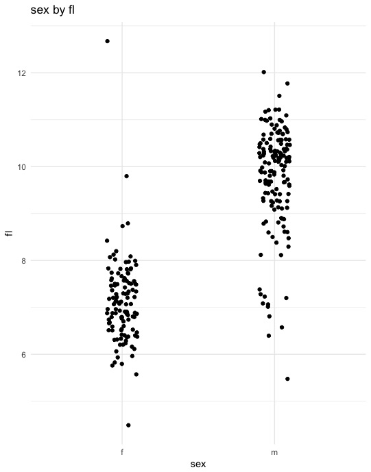
By can verify individual relationships by plotting them directly:
x %>%
  ggplot(aes(x = sex, y = fl)) +
  geom_jitter(width = 0.1) +
  theme_minimal() +
  ggtitle("sex by fl")
caveats
- complex experimental designs
If your experimental design is complicated, a pretty simplistic approach like this won’t work.
- trust but verify!
Don’t start penning your letter to Nature once you see something significant. This is really only meant to give you a sense of idea of interesting relationships. Use it to narrow down your search, then exhaustively test the most interesting relationships directly.