I went through a phase a couple weeks ago where I became obsessed with knowing everything I could about permutation / Monte Carlo / bootstrapping-based statistical methods. But besides the excellent Tidy bootstrapping with dplyr+broom I couldn’t find many resources on doing randomization-based tests in keeping with the tidy data philosophy and more modern tools for R (e.g. purrr and modelr).

At the end of the week I ended up with a lengthy R Markdown document which I figured I share in piecemeal over the coming weeks.

But first:

why? And some definitions

bootstrapping: sampling with replacement from your data. Mostly useful for getting a confidence interval or seeing the variation inherent some test statistic of interest.

permutation testing: creating all possible permutations of your data, calculating some test statistic each time to generate a null distribution of test statistics, and comparing the observed results to this distribution. Because permutation testing is often not feasible for larger datasets, I focus on the two other strategies.

Monte-Carlo sampling: Similar to permutation testing, but uses random or pseudo-random numbers to randomly permute the dataset to generate a null distribution and compare the distribution to the observed test statistic.

advantages:

makes few assumptions, especially about the form of the distribution from which the data are draw (e.g. normally distributed)
p-values are intuitive to calculate and understand
seems like magic

disadvantages:

p-values can change when you re-run the analysis (but can change less if you increase the number of times you permute the dataset)
fewer resources on running permutation tests / less entrenched in the culture of hypothesis testing

comparing two groups

Comparing some quantitative variable of interest in two groups is a common problem. For instance, many websites perform A/B testing where two different forms of a website are presented to users, data are collected, and the company then wants to know whether some user behavior differed between the two forms of the website.

Typically a two-sample t-test is used in this situation. But t-tests make a couple of assumptions that might not be true for our data. For instance, a two-sample t-test assumes that the two groups are independent, that the variance within each group is the same, and that the data within each group are normally distributed.

If we’re uncomfortable with that last assumption, it usually makes sense to use a randomization or Monte-Carlo-based approach to testing. The approach works like this:

(1) Destroy any relationship between an observation and which of the two groups it belongs to. You can think of this as taking the labels that tell you whether a given datum belongs to group 1 or group 2, shuffling them, then randomly assigning the labels to the data points.

(2) Using this new dataset with shuffled labels, compute some statistic of interest, like the difference means between the two groups.

(3) Repeat many times.

Because we’re randomly assigning the labels to the data points, it’s equally likely that each data point gets a given label; this means that this particular method assumes equal variance of the two groups. There’s a way around this assumption according to Good’s Resampling Methods: A practical guide to data analysis which I’ll cover in another post.

The difference in means in all of our permuted datasets can be thought of as our null distribution. If there’s no difference in the means between the two groups, we’d expect the difference in means we calculate from the data to fall within the middle 95% of these permuted means (assuming alpha = 0.05). We can calculate a p-value by finding the proportion of estimates in our null distribution that are more extreme than the test statistic we calculated on our dataset.

Below I show how to carry this out using a tidy data approach in R.

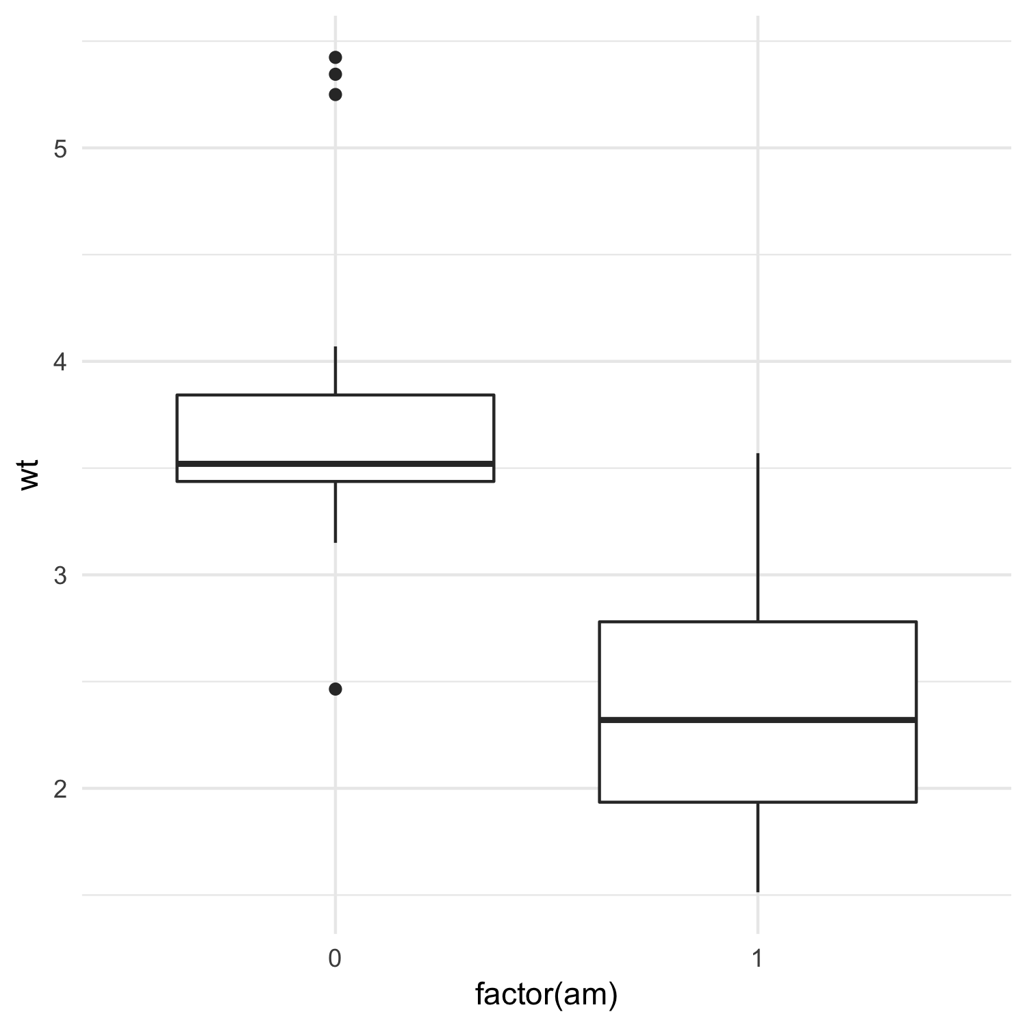
I’ll use the mtcars dataset and test whether manual and automatic cars differ in their weights:

library(tidyverse)
library(modelr)
library(broom)

mtcars %>%
  ggplot(aes(x = factor(am), y = wt)) +
  geom_boxplot() +
  theme_minimal()

We can first run a traditional two-sample t-test:

t.test(wt ~ factor(am), data = mtcars)

Welch Two Sample t-test ##
## data: wt by factor(am)
## t = 5.4939, df = 29.234, p-value = 6.272e-06
## alternative hypothesis: true difference in means is not equal to 0
## 95 percent confidence interval:
## 0.8525632 1.8632262
## sample estimates:
## mean in group 0 mean in group 1
## 3.768895 2.411000

Next we can do the randomization-based approach outlined above:

# number of permutations
n <- 999

permuted <- mtcars %>%
  mutate(am = factor(am)) %>% # factor am
  modelr::permute(n, am) %>% # permute the am column `n` times
  mutate(models = map(perm, ~ t.test(wt ~ am, data = .))) %>% # do a t-test for each permutation
  mutate(tidy = map(models, broom::glance)) %>% # extract useful statistics from the t-test
  unnest(tidy) # unnest the tidy column

permuted look like this:

# A tibble: 999 x 13
perm   .id      models     estimate estimate1 estimate2   statistic    p.value parameter    conf.low  conf.high
<list> <chr>      <list>        <dbl>     <dbl>     <dbl>       <dbl>      <dbl>     <dbl>       <dbl>      <dbl>
 1 <S3: permutation>   001 <S3: htest>  0.677473684  3.492474  2.815000  2.00328522 0.05595078  25.34094 -0.01854899  1.3734964
 2 <S3: permutation>   002 <S3: htest>  0.278704453  3.330474  3.051769  0.85140972 0.40129861  29.94857 -0.38987074  0.9472796
 3 <S3: permutation>   003 <S3: htest>  0.316016194  3.345632  3.029615  0.97431917 0.33773747  29.81439 -0.34655899  0.9785914

Each row represents a different permutation. Using broom::glance allowed us to easily pull out a bunch of useful information from the t-test, and unnesting the tidy column added these useful statistics as columns to the data frame.

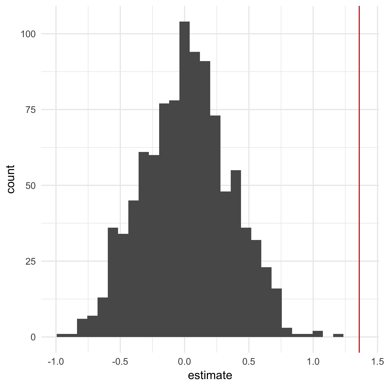
The estimate column here is the most useful to us: it represents the difference in the means between each group. If we’ve effectively destroyed any correlation between transmission type and weight, the average difference between the two groups should be zero. We can verify this is the case. I’ll also find the observed difference between the groups in the non-randomized dataset and plot that as a red line:

observed <- broom::glance(t.test(wt ~ factor(am), data = mtcars))$estimate

ggplot(permuted, aes(x = estimate)) +
  geom_histogram() +
  geom_vline(xintercept = observed, color = "red") +
  theme_minimal()

We can also calculate the average difference and show that it’s about 0 in the randomized datasets:

mean(permuted$estimate)

[1] 0.001492764

Looking at the plot above, it’s clear the the observed difference is not what we’ve expect if there is no relationship between transmission type and weight, but we can go ahead and calculate a p-value:

(sum(abs(permuted$estimate) > ifelse(observed > 0, observed, -observed)) + 1) / (n+1)

[1] 0.001

This way of calculating p-values is based on this paper and ensures p-values can never by 0, which wouldn’t make any sense.

Aside: To create randomized datasets that you can re-generate at some point in the future, use set.seed(some_number) before randomizing your data. This sets the seed of the random number generator in R, ensuring the same pseudo-random numbers are producing the next time you run your analysis.

In future posts, I’ll look at bootstrapping regressions, correlations, and using Monte-Carlo-based resampling for ANOVA-like data.